Example 2: Blazar simulation including external fields
Single-zone external field blazar model by Rodrigues et al, Astron.Astrophys. 681 (2024) A119.
The parameters used are the best-fit values for PKS 0736+01 as reported in the above paper and on this GitHub repository.
When using this model, please cite the above paper additionally to AM3.
1. Import modules and define some helper functions
[1]:
import os
import numpy as np
import pickle as pickle
import astropy.units as u
from astropy.cosmology import FlatLambdaCDM
cosmo = FlatLambdaCDM(H0=70, Om0=0.3)
from astropy.constants import codata2010 as const
from matplotlib import pyplot as plt
import seaborn as sns

import am3

def PlanckDistribution(earr, temperature, lum):
    '''
    Thermal Distribution (unnormalized)

    return: E^2dN/dE [a.u.]
    par earr (array): photon energy [eV]
    par temperature [K]
    par lum: total luminosity [erg/s]
    '''
    lgr = earr / temperature / const.k_B.to(u.eV/u.K)
    exparr = np.exp(lgr) - 1
    ednde = earr ** 4 / exparr
    integ = np.trapezoid(ednde / earr, earr)
    return ednde * lum / integ


def Schwarzschild(m_bh):
    '''Schwarzschild radius [cm]

    m_bh: black hole mass [m_solar]
    '''
    rad = (2 * const.G * m_bh * 1.989e30*u.kg
           / const.c ** 2)
    return rad.to(u.cm)


def DiskTemperature(rad, lumdisk, m_bh, eta=0.08):
    '''Radius-dependent disk temperature [K]
    '''
    sb = const.sigma_sb.to(u.erg/u.s/
                           u.K**4/u.cm**2)
    rsch = Schwarzschild(m_bh)

    term1 = 3 * rsch * lumdisk / (16 * np.pi * eta
                                  * sb * rad ** 3)
    term2 = 1 - (3 * rsch / rad) ** 0.5
    return (term1 * term2) ** 0.25


def ShakuraFlux(earr, lumdisk, m_bh, thetaobs=3.0, eta=0.08):
    '''Disk spectral flux in observer's frame [erg/cm2/s]

    earr (array): photon energies [eV]
    lumdisk: [erg/s]
    m_bh: black hole mass / m_solar
    thetaobs: angle btw. LOS and disk rotation axis (deg)
    '''
    kB = const.k_B.to(u.eV/u.K)
    c0 = const.c.cgs
    hplanck = const.h.to(u.eV*u.s)
#     dlum = cosmo.luminosity_distance(z).to(u.cm)
    rsch = Schwarzschild(m_bh)
    rin = 3 * rsch
    rout = 300 * rsch
    radarr = np.linspace(rin, rout, 50)

    frac = (4 * np.pi) ** 2 * hplanck * np.cos(thetaobs*np.pi/180) / c0 ** 2
    nuarr = earr / hplanck       # convert x-axis to obs frame
    en2d = earr[:,np.newaxis]    # convert x-axis to obs frame
    rad2d = radarr[np.newaxis,:]
    temp2d = DiskTemperature(rad2d,lumdisk,m_bh,eta) # K

    integrand = rad2d / (np.exp(en2d/temp2d/kB) - 1)
    integral = np.trapezoid(integrand, radarr, axis=1)
    Fnu = (nuarr ** 3 * frac * integral).to(u.erg)
    return nuarr * Fnu

def BroadLine(earr, center, width, lum):
    '''
    Broad line spectrum, normalized to `lum`

    return: E^2dN/dE [a.u.]
    par earr (array): photon energies (eV)
    par center: line energy [eV]
    par width: line width (eV)
    par lum: line luminosity [erg/s]
    '''
    ednde = np.exp(-0.5
                   * (earr - center) ** 2
                   / width ** 2
                  )
#     ednde[ednde < 1e-100] = 0.
    integ = np.trapezoid(ednde/earr, earr)
    ednde *= lum / integ
    return ednde

def get_BLR_density_scaling(R_zone, R_diss, lorentz):
    '''Scaling of the photon density seen in the jet frame
    with the dissipation radius, according to Eq. 20 of
    Ghisellini+Tavecchio 0902.0793
    '''

    def scaling_for_large_R_diss(R_diss, R_zone, lorentz):
        beta = (1 - 1. / lorentz ** 2) ** 0.5
        mu1 = (1 + (R_zone / R_diss) ** 2) ** -.5
        mu2 = (1 - (R_zone / R_diss) ** 2) ** .5
        f_mu = (2 * (1 - beta * mu1) ** 3
                - (1 - beta * mu2) ** 3
                - (1 - beta) ** 3)
        return f_mu / 3. / beta

    f0 = 17. / 12

    if R_diss <= R_zone:
        scaling = f0

    elif R_diss >= 3 * R_zone:
        scaling = scaling_for_large_R_diss(
            R_diss,
            R_zone,
            lorentz)

    elif R_zone < R_diss < 3 * R_zone:
        # Power-law interpolation
        f_3R = scaling_for_large_R_diss(
            3 * R_zone,
            R_zone,
            lorentz
        )
        scaling = 10 **(
            (np.log10(f_3R) - np.log10(f0))
            / (np.log10(3 * R_zone) - np.log10(R_zone))
            * (np.log10(R_diss) - np.log10(R_zone))
        )

    return scaling

def tangential_angle(R_BLR, R_diss):
    '''Calculate the characteristic angle of the radiaiton,
        which is the tangential angle. This is where the dominant
        contribution comes from because it has the highest doppler
        boost, as well as for geometric reasons.
    '''
    csi = np.arcsin(R_BLR/R_diss)
    return csi

def calc_doppler(lorentz, R_BLR, R_diss):
    '''Calculate relative Doppler factor between blob and BLR.
        The blob has bulk factor `lorentz` and distance to the black hole
        given by `R_diss` [cm]. The BLR has radius `R_BLR` [cm].
    '''
    if R_diss <= R_BLR:
        return lorentz

    csi = tangential_angle(R_BLR, R_diss)
    beta = (1 - 1. / lorentz ** 2) ** 0.5
    doppler = lorentz * (1 - beta * np.cos(csi))
    return doppler

def convert_lum_to_density_in_jet(R_diss, lorentz, R_BLR):
        ''' Convert external field luminosity in the rest frame of the
        black hole in [erg/s] into energy density in the comoving frame
        of the jet blob in [GeV / cm^3]. R_BLR can represent the BLR radius
        or the dust torus radius.

        This is an *approximation where the emission is considered to come
        only from the tangential direction*. See Fig. 1 of Ghisellini and
        Tavecchio 2009 (arXiv:0902.0793)

        return: conversion factor [GeV erg^-1 s cm^-3]
        '''

        f1 = (lorentz ** 2 # In a previous version of the notebook,
                           # this line read (Doppler factor) ** 2.
                           # This is the correct expression.
                / (4.
                    * np.pi
                    * R_BLR ** 2
                    * const.c.cgs.value)
                * u.erg.to('GeV'))

        f2 = get_BLR_density_scaling(R_BLR, R_diss, lorentz)
        factor =  f1 * f2

        return factor
This should be done only once every time you import the AM3 module.
Once you initialize AM3, the same kernel can be used for subsequent simulations.
To inject different particle distributions, simply do am3.clear_particle_densities() and inject the new ones. This does not require a kernel recomputation.
To change the magnetic field, use am3.set_mag_field(new_bfield). This triggers a kernel re-compuation.
[2]:
%%time

# Initialize the AM3 module
am3 = am3.AM3()

# Adjust min photon energy, min neutrino energy, and max energy for all particles [eV].
# This allows us to optimize the performance depending on the needs of the specific science case
am3.update_energy_grid(1e-6, 1e3, 1e18)

# Manually define max proton and electron energy
am3.set_estimate_max_energies(0)

# Turn on for keeping track of the different SED components, for plotting purposes;
# turn off for efficiency.
am3.set_process_parse_sed(1)

# Hadronic processes on
am3.set_process_hadronic(1)

# Keep track of positrons and electrons separately
am3.set_process_merge_positrons_into_electrons(0)

# Escape (see documentation)
am3.set_process_escape(1)

# Expansion of radiation zone (see documentation). This one is stationary.
am3.set_process_expansion(0)
am3.set_process_adiabatic_cooling(0)

# Electron synchrotron and synchrotron self-absorption
am3.set_process_electron_syn(1)
am3.set_process_ssa(1)

# Proton synchrotron - subdominant in this case, but may be relevant for B>~10 G
am3.set_process_proton_syn(1)

# Quantum synchrotron for pairs off by default.
# In AGN simulations this effect can typically be neglected, so turn off for efficiency
am3.set_process_quantum_syn(0)

# Inverse Compton by electrons and protons
am3.set_process_electron_compton(1)
am3.set_process_proton_compton(1)

# Direct Compton turned off by default
am3.set_process_compton_photon_energy_loss(0)


# Synchrotron and inverse Compton by muons and pions - off by default.
# In AGN simulations this effect can typically be neglected, so turn off for efficiency
am3.set_process_muon_syn(0)
am3.set_process_pion_syn(0)
am3.set_process_muon_compton(0)
am3.set_process_pion_compton(0)

# Secondary particle decay
am3.set_process_pion_decay(1)
am3.set_process_muon_decay(1)

# Photon annihilation (gamma gamma -> e- e+)
am3.set_process_annihilation(1)
am3.set_optimize_annihilation_pair_emission(1) # optimization

# Bethe-Heitler pair production (p gamma -> p e+ e-)
am3.set_process_bethe_heitler(1)
am3.set_optimize_bethe_heitler_outgoing_pairs_grid(1)
am3.set_optimize_bethe_heitler_incoming_protons_min(1e12)
am3.set_optimize_bethe_heitler_target_photon_max(1e6)

# Photo-pion production (nucleon gamma -> nucleon pion)
am3.set_process_photopion(1)
am3.set_optimize_photopion_target_photon_grid(1)
am3.set_optimize_photopion_target_photon_max(1e6)

am3.set_profile_timing(1) # Used for profiling, as in the bottom plot. Turn off for efficiency.

# Initialize the AM3 kernels with the above settings
am3.init_kernels()
init. AM3 kernels:
CPU times: user 8.27 s, sys: 210 ms, total: 8.48 s
Wall time: 4.49 s
AM3 has the following switches (at step: 0)
estimate maximum energies: 0
parse sed components: 1
escape: 1
expansion: 0
adiabatic: 0
synchrotron:
  e+/-: 1  (em..: 1, cool.: 1)
  protons:1  (em..: 1, cool.: 1)
  pions:0  (em..: 1, cool.: 1)
  muons:0  (em..: 1, cool.: 1)
  syn-self-abs.:1
  e+/- quantum-syn.:0
inv. Compton:
  e+/-: 1  (em.. : 1, cool.: 1 (continuous))
  photon loss due to upscattering: 0
  protons:1  (em.. (step approx.): 1, no cooling)
  pions:0  (em.. (step approx.): 1, cont. cool.: 1)
  muons:0  (em.. (step approx.): 1, cont. cool.: 1)
pair prod. (gamma+gamma->e+e)1  (photon loss.: 1, e+/- source (feedback): 1(opt. 14-bin kernel))
'hadronic' processes (below): 1
 Pion decay: 1 Muon decay:1)
proton Bethe-Heitler: 1  (em..: 1, cool.: 1)
proton photo-pion: 1  (em..: 1, cool.: 1, photon loss: 1)
proton p-p: 1  (em..: 1 , cool.: 1)

AM3 params (comoving):
escape_timescale: 1e+06 s
  with fractions: (protons: 1, neutrons: 1, pions: 1, muons: 1, neutrinos: 1, pairs: 1)
expansion_timescale: 1e+06 s
t_adi: 3e+06 s
B: 0.01 G
pp target density = 0 cm^-3
dt = 1000 s
eta_Bohm: electrons:1, protons: 1
inj. el:
  power density = 0 erg/s/cm^3,
   Emin = 1e+07 eV,
   Ebreak = 1e+07 eV,
   Emax = 1e+13 eV,
   index = 2,
   index above break = 2,
   cut_off steepness = 1
inj. protons: power density = 0 erg/s/cm^3,
   Emin = 1e+10 eV,
   Ebreak = 1e+10 eV,
   Emax = 1e+15 eV,
   index = 2,
   index above break = 2,
   cut_off steepness = 1
and update the magnetic field strength and the light-crossing time in AM3 basde on the defined values
[12]:
pars = {

    # Parameters describing the single-zone geometry
    'r_blob' :   4.62e+16, # cm
    'magfield' : 0.783, # gauss
    'lorentz' :  17.6, # Jet bulk Lorentz factor (impacts both the relativistic boosting
                      # of the external fields into the jet frame and the boost of the jet
                      # emission into the observer's frame)
    'rdiss' :    3.42e+17, # Dissipation radius in cm (cf Fig.2 of Rodrigues+2023)
                          # (impacts the density and relativistic boost of the
                          # external fields in the jet rest frame)

    # Electron injection
    # (in this case we assume a single power-law spectrum, see below)
    'elec_emin' :  2.16e1 * (const.m_e * const.c ** 2).to(u.eV).value, # eV
    'elec_emax' :  7.36e3 * (const.m_e * const.c ** 2).to(u.eV).value, # eV
    'eindex' :     2.02,
    'elum' :       1.84e+41, # erg/s

    # Proton injection
    # (in this case we assume a single power-law spectrum, see below)
    'proton_emin' :  1e2 * (const.m_p * const.c ** 2).to(u.eV).value, # eV
    'proton_emax' :  2e6 * (const.m_p * const.c ** 2).to(u.eV).value, # eV
    'pindex' :       1.0,
    'plum' :         6.29e+43, # erg/s

    # Other source parameters

    'z' : 0.19,
    'disk_lum' :  1e45 * u.erg/u.s, # accretion disk luminosity
    'black_hole_mass' : 6e8, # [solar mass units]

    'torus_temperature' : 500 * u.K,
    'blr_covering' : 0.1,
    'torus_covering' : 0.3
    }


# Below, we calculate the size of the BLR and torus and the relative Doppler
# factor of the external photons into the jet frame based on the above parameters

pars['blr_radius'] = 1e17 * (pars['disk_lum'].value / 1e45) ** 0.5  # [cm]
pars['torus_radius'] = 2.5e18 * (pars['disk_lum'].value / 1e45) ** 0.5 # [cm]
pars['blr_doppler'] = calc_doppler(pars['lorentz'], pars['blr_radius'], pars['rdiss'])
pars['torus_doppler'] = calc_doppler(pars['lorentz'],pars['torus_radius'],pars['rdiss'])

# Set homogeneous magnetic field strength
am3.set_mag_field(pars['magfield'])

# Set escape time scale (subject to escape switch - in this case escape is on)
am3.set_escape_timescale(pars['r_blob'] / const.c.cgs.value) # 4.62e16 cm == Size of the region

# Set solver time step, in this case one-tenth of the light-crossing time
am3.set_solver_time_step(1e-1 * am3.get_escape_timescale())

# Note 1:
# All the above parameters can be changed at any time during runtime. However,
# make sure to check where each parameter is used and update it accordingly.
# For example, the B-field strength is used only internally by AM3, so changing
# its value requires calling `am3.set_mag_field(new_value)`. The blob size, r_blob,
# is used internally by AM3 (for the escape rate) as well as externally (to
# calculate the particle densities in the cell below). The bulk Lorentz factor enters
# the calculation of the external fields as well as the flux in the observer's
# frame, etc.

# Note 2:
# The escape timescale would control adiabatic cooling losses as well as the reduction in particle density
# due to the expansion of the region.
# In this example, both processes are turned off because we simulate a stationary region, so there is
# no need to define it.
# am3.set_expansion_timescale(4.62e+16 / const.c.cgs.value)

# Note 3:
# The solver time step define above is quite large, and it leads to accurate results
# only for optically thin sources (e.g. most single-zone blazar models). For more
# extreme environments, it may be necessary to decrease the solver time step
# to capture the numerical hardness of the equations. As a rule of thumb, we want to
# look at the fastest process rates at the relevant particle energies.
Set magnetic field strength and escape timescale (light-crossing time of the region)
Additionally to the general escape timescale, the escape rate of each species can be individually adjusted.
For example, doing am3.set_escape_fraction_charged_particles(0.01) decreases the escape rate of charged particles by a factor 100.
Create arrays with the accelerated electron and proton spectra
This is an example of the most generic way to inject any user-defined electron and proton spectra.
For the specific case of simple or broken power law injection, the same can also be achieved with the template function provided in AM3. For example:
volume = 4./3 * np.pi * (am3.get_escape_timescale() * const.c.cgs.value) ** 3
am3.set_powerlaw_injection_parameters_electrons(volume, elum, elec_emin, elec_emin, elec_emax, eindex, eindex, 1.0)
[ ]:
# Create electron spectrum, in this case a simple power law.
# The same can also be achieved using the template powerlaw function:
# am3.set_electron_powerlaw_injection_parameters_parameters((elum, elec_emin, elec_emin, elec_emax, eindex, eindex, 1.0))

egrid = am3.get_egrid_lep()
epowerlaw = (egrid ** (2 - pars['eindex'])
                * (egrid >= pars['elec_emin'])
                * np.exp(- egrid / pars['elec_emax'])
            )
# Integrate spectrum in erg/s
etrapz = np.trapezoid(epowerlaw / egrid, egrid)

# Normalize it to the desired electron lumiosity
enormalized = epowerlaw * pars['elum'] / etrapz # erg/s

# Convert it to an energy density injection rate
volume = 4/3 * np.pi * pars['r_blob'] ** 3
enormalized /= volume # erg/cm3/s

# And finally to a particle density injection rate
enormalized /= egrid * u.eV.to(u.erg) # cm-3.s-1


# Create proton spectrum, in this case also a simple power law.
# The same can be achieved using the template powerlaw function:
# io.set_proton_powerlaw_injection_parameters_parameters((plum, proton_emin, proton_emin, proton_emax, pindex, pindex, 1.0))

pgrid = am3.get_egrid_had()
ppowerlaw = (pgrid ** (2 - pars['pindex'])
                * (pgrid >= pars['proton_emin'])
                * np.exp(- pgrid / pars['proton_emax'])
            )

# Integrate spectrum in erg/s
ptrapz = np.trapezoid(ppowerlaw / pgrid, pgrid)

# Normalize it to the desired proton lumiosity
pnormalized = ppowerlaw * pars['plum'] / ptrapz # erg/s

# Convert it to an energy density injection rate
volume = 4/3 * np.pi * pars['r_blob'] ** 3
pnormalized /= volume # erg/cm3/s

# And finally to a particle density injection rate
pnormalized /= pgrid * u.eV.to(u.erg) # cm-3.s-1
Define external photon spectrum
In this case we consider three components (see Fig. 2 of Rodrigues+ 2023):
Broad lines from hydrogen and helium Lymann alpha emission
Fraction of the thermal disk emission scattered in the BLR (following a multi-temperature Shakura-Sunaev spectrum)
Infrared emission from a dust torus (following a simple black-body spectrum)
Below we define arrays with the spectral shapes of these different components, normalize them to the disk luminosity including the respective covering factors, boost them into the jet rest frame, add them up into a single array, and finally inject this in the simulation as external photons.
[5]:
# AM3 photon grid
egrid_jetframe = am3.get_egrid_photons() * u.eV

# Set up array for adding up external fields
external_photons = np.zeros(egrid_jetframe.size) * u.GeV / u.cm**3

# Scattered thermal disk emission
disky = ShakuraFlux(egrid_jetframe / pars['blr_doppler'],
                    pars['disk_lum'],
                    pars['black_hole_mass'],
                    3.0) # erg/s, black hole frame

# Broad line emission
hybl = BroadLine(egrid_jetframe / pars['blr_doppler'],
                    10.2*u.eV, 10.2*u.eV/20, # H Ly alpha line energy and width
                    pars['disk_lum'] * pars['blr_covering']) # [erg/s]
hebl = BroadLine(egrid_jetframe / pars['blr_doppler'],
                    40.8*u.eV, 40.8*u.eV/20, # He Ly alpha line energy and width
                    pars['disk_lum'] * pars['blr_covering'] * 0.5) # [erg/s]
# Convert BLR components to jet frame
blr_to_jet = convert_lum_to_density_in_jet(pars['rdiss'],
                                           pars['lorentz'],
                                           pars['blr_radius']) # erg/s -> GeV/cm3
blr_to_jet *= u.GeV / u.cm ** 3 / (u.erg / u.s) # give it units

blr_pho = (disky * 0.01 + hybl + hebl) * blr_to_jet # GeV/cm3

external_photons += blr_pho

# Dust torus
torusy = PlanckDistribution(egrid_jetframe / pars['torus_doppler'],
                            pars['torus_temperature'],
                            pars['disk_lum'] * pars['torus_covering']) # [erg/s]
# Convert torus emission to jet frame
tor_to_jet = convert_lum_to_density_in_jet(pars['rdiss'],
                                           pars['lorentz'],
                                           pars['torus_radius']) # erg/s -> GeV/cm3
tor_to_jet *= u.GeV / u.cm**3 / (u.erg/u.s)  # give it units
# Add torus to BLR components
torus_pho = torusy * tor_to_jet
external_photons += torus_pho

# Convert summed up components from energy density to photon density in jet frame
external_photonspectrum = (external_photons / egrid_jetframe).to(u.cm ** -3).value # cm-3

# Convert photon density to density ijnjection rate
external_photonspectrum /= am3.get_escape_timescale() # cm-3.s-1
/opt/anaconda3/envs/am3/lib/python3.12/site-packages/astropy/units/quantity.py:659: RuntimeWarning: divide by zero encountered in divide
  result = super().__array_ufunc__(function, method, *arrays, **kwargs)
/opt/anaconda3/envs/am3/lib/python3.12/site-packages/astropy/units/quantity.py:659: RuntimeWarning: overflow encountered in exp
  result = super().__array_ufunc__(function, method, *arrays, **kwargs)
Inject electron, proton and photon arrays defined above into the simulation.
The next two cells can be re-run with the same kernel to simulate different particle distributions with the same magnetic field.
[6]:
%%time
# Reset all particle arrays to zero
am3.clear_particle_densities()
# Inject cosmic rays and external photons in the simulation
am3.set_injection_rate_electrons(enormalized)
am3.set_injection_rate_protons(pnormalized)
am3.set_injection_rate_photons(external_photonspectrum)
# Start the system with correct initial external photon density
# (this should not strongly affect the steady-state result)
am3.set_current_densities_photons(external_photonspectrum * am3.get_escape_timescale())
saved_photons = am3.get_photons()
# Plot injection rates
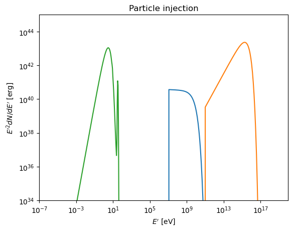
density_injection_rate_to_luminosity = 4 * np.pi / 3 * am3.get_escape_timescale() ** 3 * const.c.cgs.value ** 3 * u.eV.to(u.erg) # eV/cm3-> erg/s
plt.loglog(am3.get_egrid_lep(), am3.get_injection_rate_electrons() * am3.get_egrid_lep() * density_injection_rate_to_luminosity)
plt.loglog(am3.get_egrid_had(), am3.get_injection_rate_protons() * am3.get_egrid_had() * density_injection_rate_to_luminosity)
plt.loglog(am3.get_egrid_photons(), am3.get_injection_rate_photons() * am3.get_egrid_photons() * density_injection_rate_to_luminosity)
plt.axis([1e-7,1e20,1e34,1e45])
plt.xlabel(r'$E^\prime$ [eV]')
plt.ylabel(r'$E^{\prime2} dN/dE^\prime$ [erg]')
plt.title("Particle injection")
plt.show()
CPU times: user 188 ms, sys: 10.9 ms, total: 199 ms
Wall time: 213 ms
Run simulation
[7]:
%%time

profiling = []

time = 0.
while time < 3 * am3.get_escape_timescale(): # Run up to 3x the light-crossing time a
    am3.evolve_step() # Evolve solver
    time += am3.get_solver_time_step() # Count time
    profiling.append(am3.get_profiled_times()) # Add computation times for profiling
CPU times: user 694 ms, sys: 9.06 ms, total: 703 ms
Wall time: 353 ms
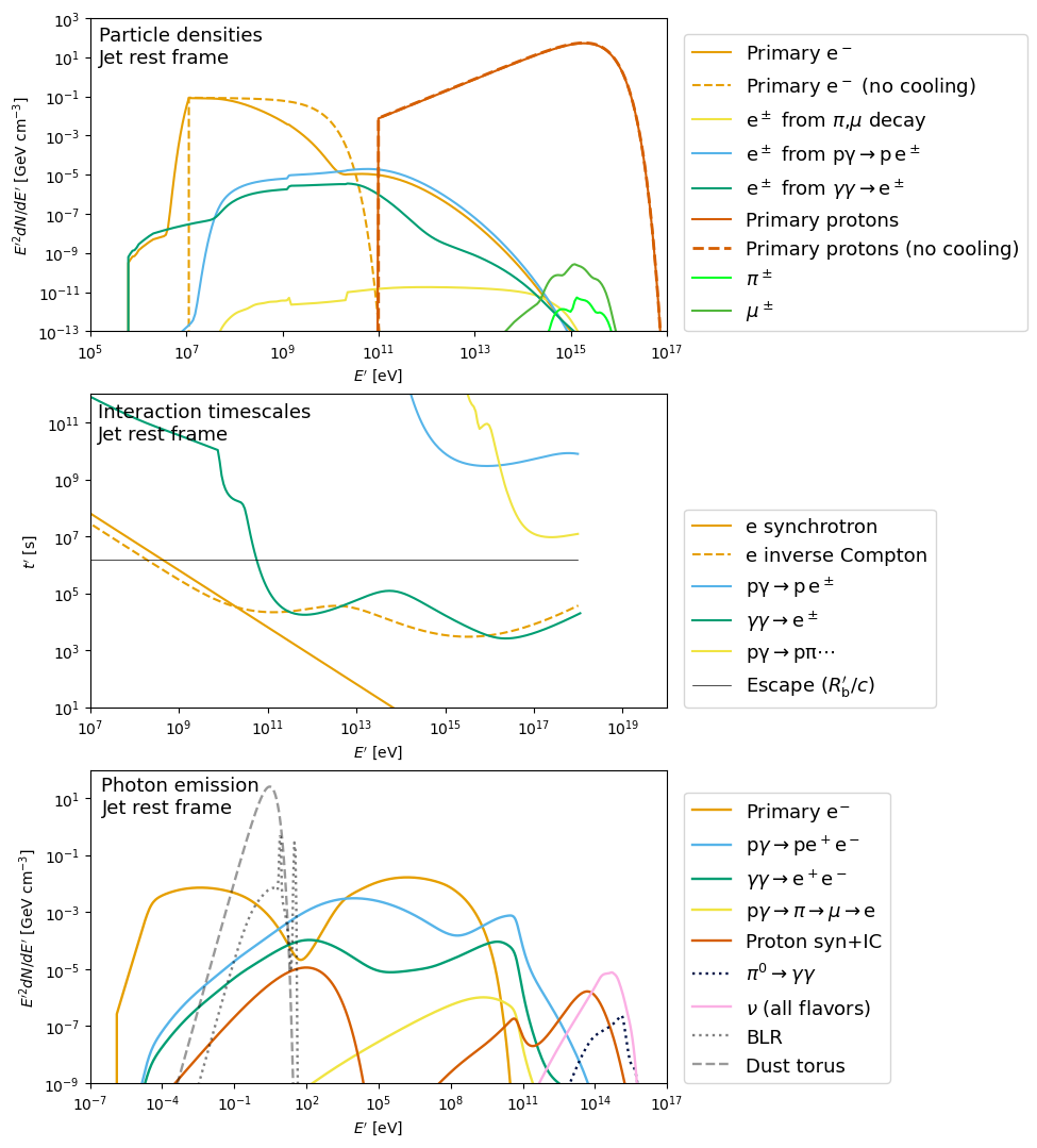
5. Plot results
Particle densities and interaction rates in the source rest frame
[8]:
mycolors = np.array([np.array([230,159,  0.]),
                     np.array([ 86,180,233.]),
                     np.array([  0,158,115.]),
                     np.array([240,228, 66.]),
                     np.array([  0,114,178.]),
                     np.array([213, 94,  0.]),
                     np.array([201,121,176.])])
mycolors *= 1./255

fig, axs = plt.subplots(3, 1, figsize=(7, 13)) # , gridspec_kw={'width_ratios': [1,1]}

##############
## Particle densities
##############

ax1 = axs[0]
plt.sca(ax1)


egrid_ele = am3.get_egrid_lep()
egrid_had = am3.get_egrid_had()


ele_mass = (const.m_e * const.c ** 2).cgs.to(u.eV).value
pro_mass = (const.m_p * const.c ** 2).cgs.to(u.eV).value

colors = sns.color_palette("hsv", n_colors=10)
color_ele_primary = colors[-1]
color_ele_secondary = colors[-2]
color_pro = colors[5]

color_muon = sns.xkcd_rgb['leafy green']
color_pion = colors[-7]


plt.loglog(egrid_ele,
           am3.get_electrons() * egrid_ele*u.eV.to(u.GeV),
           c=mycolors[0],
           label='Primary e$^-$')
plt.loglog(egrid_ele,
           am3.get_injection_rate_electrons() * egrid_ele*u.eV.to(u.GeV) * am3.get_escape_timescale(),
           c=mycolors[0], ls='--',
           label='Primary e$^-$ (no cooling)')
plt.loglog(egrid_ele,
           am3.get_pairs_photopion() * egrid_ele * u.eV.to(u.GeV),
           c=mycolors[3],
           label=r'e$^\pm$ from $\pi$,$\mu$ decay')

plt.loglog(egrid_ele,
           am3.get_pairs_bethe_heitler() * egrid_ele * u.eV.to(u.GeV),
           c=mycolors[1],
           label=r'e$^\pm$ from $\rm{p}\gamma\rightarrow \rm{p}\,\rm{e}^\pm$')


plt.loglog(egrid_ele,
           am3.get_pairs_annihilation() * egrid_ele * u.eV.to(u.GeV),
           c=mycolors[2],
           label=r'e$^\pm$ from $\gamma\gamma\rightarrow \rm{e}^\pm$')


plt.loglog(egrid_had,
           am3.get_protons() * egrid_had*u.eV.to(u.GeV) ,
           c=mycolors[5],
           label='Primary protons')

plt.loglog(egrid_had,
           am3.get_injection_rate_protons() * egrid_had*u.eV.to(u.GeV) * am3.get_escape_timescale(),
           c=mycolors[5],
           ls='--',
           lw=2,
           label='Primary protons (no cooling)')

plt.loglog(egrid_had,
           am3.get_pions() * egrid_had * u.eV.to(u.GeV),
           c=color_pion, ls='-',
           label=r'$\pi^\pm$')


plt.loglog(egrid_had,
           am3.get_muons() * egrid_had * u.eV.to(u.GeV),
           c=color_muon, ls='-',
           label=r'$\mu^\pm$')

plt.annotate("Particle densities\nJet rest frame",
             (1.5e5,4e2),
             fontsize=13,
             horizontalalignment='left',
             verticalalignment='top')

plt.legend(loc=(0,0),ncol=1,bbox_to_anchor=(1.03,0),fontsize=13)
plt.xlabel(r"$E^\prime$ [eV]")
plt.ylabel(r"$E^{\prime2} dN/dE^\prime$ [GeV cm$^{-3}$]")
plt.axis([1e5,1e17,1e-13,1e3])


##############
## Timescales
##############

ax2 = axs[1]
plt.sca(ax2)


egrid_ele = am3.get_egrid_lep()
egrid_pro = am3.get_egrid_had()
egrid_pho = am3.get_egrid_photons()

ele_mass = (const.m_e * const.c ** 2).cgs.to(u.eV).value
pro_mass = (const.m_p * const.c ** 2).cgs.to(u.eV).value

colors = sns.color_palette("hsv", n_colors=10)
color_ele_primary = colors[-1]
color_ele_secondary = colors[-2]
color_pro = colors[5]

color_muon = colors[-10]
color_pion = colors[-7]


plt.loglog(egrid_ele,
           am3.get_t_pair_syn(),
           c=mycolors[0],
           label='e synchrotron')
plt.loglog(egrid_ele,
           am3.get_t_pair_compton(),
           c=mycolors[0], ls='--',
           label='e inverse Compton')

plt.loglog(egrid_had,
           am3.get_t_proton_bethe_heitler(),
           c=mycolors[1],
           label=r'$\rm{p}\gamma\rightarrow \rm{p}\,\rm{e}^\pm$')

plt.loglog(egrid_pho,
           am3.get_t_photon_annihilation(),
           c=mycolors[2],
           label=r'$\gamma\gamma\rightarrow \rm{e}^\pm$')

plt.loglog(egrid_had,
           am3.get_t_proton_photopion(),
           c=mycolors[3],
           label=r'$\rm{p}\gamma\rightarrow \rm{p}\pi\cdots$')

plt.loglog([egrid_ele[0], egrid_had[-1]],
           np.full(2, am3.get_escape_timescale()),
           c='k',
           lw=0.5,
           label=r'Escape ($R_\mathrm{b}^\prime/c$)')


plt.annotate("Interaction timescales\nJet rest frame",
             (1.5e7,5e11),
             fontsize=13,
             horizontalalignment='left',
             verticalalignment='top')

plt.legend(loc=(0,0),ncol=1,bbox_to_anchor=(1.03,0),fontsize=13)
plt.xlabel(r"$E^\prime$ [eV]")
plt.ylabel(r"$t^\prime$ [s]")
plt.axis([1e7,1e20,1e1,1e12])


##############
## Jet frame SED
##############

ax3 = axs[2]
plt.sca(ax3)


# Energy arrays in source frame
egrid_pho = am3.get_egrid_photons()
egrid_nu = am3.get_egrid_neutrinos()

# Get individual SED components

all_nu = am3.get_neutrinos() * egrid_nu * u.eV.to(u.GeV)
external_pho = am3.get_injection_rate_photons() * am3.get_escape_timescale() *  egrid_pho * u.eV.to(u.GeV)
injected = am3.get_photons_injected_electrons_syn_compton() * egrid_pho * u.eV.to(u.GeV)
annihil = am3.get_photons_annihilation_pairs_syn_compton() * egrid_pho * u.eV.to(u.GeV)
all_photons = am3.get_photons() * egrid_pho * u.eV.to(u.GeV)
bheitler = am3.get_photons_bethe_heitler_pairs_syn_compton() * egrid_pho * u.eV.to(u.GeV)
pgamma = am3.get_photons_photo_pion_pairs_syn_compton() * egrid_pho * u.eV.to(u.GeV)
pi0decay = am3.get_photons_pi0_decay() * egrid_pho * u.eV.to(u.GeV)
proton_syn_ic = am3.get_photons_protons_syn_compton() * egrid_pho * u.eV.to(u.GeV)


# Create plot


# Plot components
plt.loglog(egrid_pho, injected,
            c=mycolors[0],
            lw=1.7,
            label=r'Primary e$^{-}$')
plt.loglog(egrid_pho, bheitler,
            c=mycolors[1],
            lw=1.7,
            label=r'p$\gamma\rightarrow$pe$^+$e$^-$')

plt.loglog(egrid_pho, annihil,
            c=mycolors[2],
            lw=1.7,
            label=r'$\gamma\gamma\rightarrow$e$^+$e$^-$')
plt.loglog(egrid_pho, pgamma,
            c=mycolors[3],
            lw=1.7,
            label=r'p$\gamma\rightarrow\pi\rightarrow\mu\rightarrow$e')
plt.loglog(egrid_pho, proton_syn_ic,
            c=mycolors[5],
            lw=1.7,
            label='Proton syn+IC')
plt.loglog(egrid_pho, pi0decay,
            c=sns.xkcd_rgb['navy blue'],
            ls=':',lw=1.7,
            label=r'$\pi^0\rightarrow\gamma\gamma$')

# Plot all-flavor neutrino spectrum
plt.loglog(egrid_nu, all_nu, label=r'$\nu$ (all flavors)',
           lw=1.7, color=sns.color_palette("colorblind",12)[6])


# Plot external photons
plt.loglog(egrid_pho, blr_pho, # obs frame, erg/cm2/s
           lw=1.7, c='k', ls=':',alpha=0.5,label=r'BLR')
plt.loglog(egrid_pho, torus_pho, # obs frame, erg/cm2/s
           lw=1.7, c='k', ls='--',alpha=0.4,label=r'Dust torus')

plt.xlabel(r"$E^\prime$ [eV]")
plt.ylabel(r"$E^{\prime2} dN/dE^\prime$ [GeV cm$^{-3}$]")
plt.axis([1e-7,1e17,1e-9,1e2])

plt.annotate("Photon emission\nJet rest frame",
             (3e-7,6e1),
             fontsize=13,
             horizontalalignment='left',
             verticalalignment='top')

plt.legend(loc=(1.03,0), fontsize=13,frameon=1,ncol=1)

plt.tight_layout(rect=(0.5,0,1,1))

plt.savefig("blazar_plots.png",dpi=300,bbox_inches='tight')

plt.show()
/var/folders/25/d230kxr90hj414fnx8hg1f_4000956/T/ipykernel_31055/1099422938.py:244: UserWarning: Tight layout not applied. The left and right margins cannot be made large enough to accommodate all Axes decorations.
  plt.tight_layout(rect=(0.5,0,1,1))
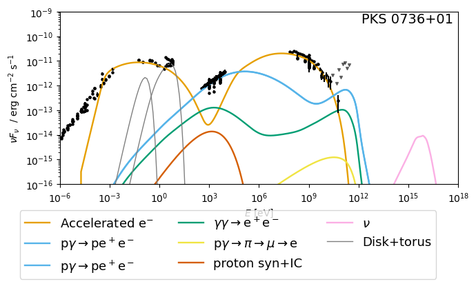
Multi-wavelength fluxes in the observer’s frame, including EBL attenuation
[9]:
# ##########################################
# Import EBL attenuation cutoff from gammapy
# ##########################################

# Download data

import requests
url = 'https://github.com/gammapy/gammapy-extra/raw/master/datasets/ebl/ebl_dominguez11.fits.gz'

os.makedirs('data/ebl', exist_ok=True)
local_filename = 'data/ebl/ebl_dominguez11.fits.gz'

response = requests.get(url)
with open(local_filename, 'wb') as f:
    f.write(response.content)

print(f"EBL data downloaded from gammapy-extras and saved as {local_filename}")

# Implement Spectral attenuation model

from gammapy.modeling.models import (
    EBLAbsorptionNormSpectralModel,
    Models,
    PowerLawSpectralModel,
    SkyModel,
)
os.environ["GAMMAPY_DATA"] = "./data/"
dominguez = EBLAbsorptionNormSpectralModel.read_builtin("dominguez", redshift=0.)

# ##################
# Conversion factors
# ##################

# Jet frame -> obs. frame
energy_conversion = pars['lorentz'] / (1 + pars['z'])

# erg/cm3, source frame -> erg/cm2/s, obs. frame
lum_dist = cosmo.luminosity_distance(pars['z']).cgs.value
density_to_lum = 4 * np.pi * pars['r_blob'] ** 2 * const.c.cgs.value
lum_to_flux = 1./(4 * np.pi * lum_dist ** 2)
spectrum_conversion = density_to_lum * lum_to_flux * pars['lorentz'] ** 4

# Energy arrays in source frame
egrid_pho = am3.get_egrid_photons()
egrid_nu = am3.get_egrid_neutrinos()

# Energy arrays in observer's frame
egrid_pho_obs = egrid_pho * energy_conversion
egrid_nu_obs = egrid_nu * energy_conversion

# Implement attenuation
atten = dominguez.evaluate(egrid_pho_obs * u.eV, pars['z'], 1.0)

# ######################################
# Get individual SED components from AM3
# ######################################

all_nu = am3.get_neutrinos() * egrid_nu * u.eV.to(u.erg) * spectrum_conversion
external_pho = am3.get_injection_rate_photons() * am3.get_escape_timescale() *  egrid_pho * u.eV.to(u.erg) * spectrum_conversion * atten
injected = am3.get_photons_injected_electrons_syn_compton() * egrid_pho * u.eV.to(u.erg) * spectrum_conversion * atten
annihil = am3.get_photons_annihilation_pairs_syn_compton() * egrid_pho * u.eV.to(u.erg) * spectrum_conversion * atten
bheitler = am3.get_photons_bethe_heitler_pairs_syn_compton() * egrid_pho * u.eV.to(u.erg) * spectrum_conversion * atten
pgamma = am3.get_photons_photo_pion_pairs_syn_compton() * egrid_pho * u.eV.to(u.erg) * spectrum_conversion * atten
pi0decay = am3.get_photons_pi0_decay() * egrid_pho * u.eV.to(u.erg) * spectrum_conversion * atten
proton_syn_ic = am3.get_photons_protons_syn_compton() * egrid_pho * u.eV.to(u.erg) * spectrum_conversion * atten


# ###########
# Create plot
# ###########

_ = plt.figure(figsize=(7,5))

mycolors = np.array([np.array([230,159,  0.]),
                     np.array([ 86,180,233.]),
                     np.array([  0,158,115.]),
                     np.array([240,228, 66.]),
                     np.array([  0,114,178.]),
                     np.array([213, 94,  0.]),
                     np.array([201,121,176.])])
mycolors *= 1./255

# Plot components
plt.loglog(egrid_pho_obs, injected,
            c=mycolors[0],
            lw=1.7,
            label=r'Accelerated e$^{-}$')

plt.loglog(egrid_pho_obs, bheitler,
            c=mycolors[1],
            lw=1.7,
            label=r'p$\gamma\rightarrow$pe$^+$e$^-$')

plt.loglog(egrid_pho_obs, bheitler,
            c=mycolors[1],
            lw=1.7,
            label=r'p$\gamma\rightarrow$pe$^+$e$^-$')


plt.loglog(egrid_pho_obs, annihil,
            c=mycolors[2],
            lw=1.7,
            label=r'$\gamma\gamma\rightarrow$e$^+$e$^-$')


plt.loglog(egrid_pho_obs, pgamma,
            c=mycolors[3],
            lw=1.7,
            label=r'p$\gamma\rightarrow\pi\rightarrow\mu\rightarrow$e')

plt.loglog(egrid_pho_obs, proton_syn_ic,
            c=mycolors[5],
            lw=1.7,
            label='proton syn+IC')

# # Gamma rays from pi zeros are attenuated in EBL interactions
# plt.loglog(egrid_pho_obs, pi0decay,
#             c='gray',
#             ls=':',lw=1.7,
#             label=r'$\pi^0\rightarrow\gamma\gamma$')

# Plot all-flavor neutrino spectrum
plt.loglog(egrid_nu_obs, all_nu, label=r'$\nu$',
            lw=1.7, color=sns.color_palette("colorblind",12)[6])

# Plot thermal emission

ethermal = np.logspace(-3,3,50)
eobs = ethermal / (1 + pars['z'])
disk = ShakuraFlux(ethermal * u.eV,
                    pars['disk_lum'],
                    pars['black_hole_mass']
                    ) * lum_to_flux

torus = PlanckDistribution(ethermal * u.eV,
                            500 * u.K,
                            pars['disk_lum'] * pars['torus_covering'] * u.erg/u.s
                            ) * lum_to_flux

plt.loglog(eobs, disk, color='gray',lw=1.0,label='Disk+torus')
plt.loglog(eobs, torus, color='gray',lw=1.0)

plt.xlabel(r"$E$ [eV]")
plt.ylabel(r"$\nu F_\nu$  / erg cm$^{-2}$ s$^{-1}$")
plt.axis([1e-6,1e18,1e-16,1e-9])

plt.annotate("PKS 0736+01",
(5e17,3.5e-10),
fontsize=14,
horizontalalignment='right')

plt.legend(loc=(-0.1,-0.55), fontsize=13,frameon=1,ncol=3)

data_x, data_y, data_err, uplims_x, uplims_y = np.load('data/data_pks_0736+01.npy', allow_pickle=1)

plt.scatter(data_x, data_y, s=5, c='k')
plt.errorbar(data_x, data_y, data_err, ls='none',c='k')
plt.scatter(uplims_x, uplims_y, s=8,c='k',alpha=0.5,marker="v")

plt.tight_layout()


plt.show()
EBL data downloaded from gammapy-extras and saved as data/ebl/ebl_dominguez11.fits.gz
/opt/anaconda3/envs/am3/lib/python3.12/site-packages/astropy/units/quantity.py:659: RuntimeWarning: divide by zero encountered in divide
  result = super().__array_ufunc__(function, method, *arrays, **kwargs)
/opt/anaconda3/envs/am3/lib/python3.12/site-packages/astropy/units/quantity.py:659: RuntimeWarning: overflow encountered in exp
  result = super().__array_ufunc__(function, method, *arrays, **kwargs)
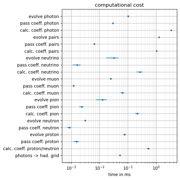
6. Profiling
[11]:
# This requires the switch
fig, ax = plt.subplots(figsize=(6,6))
rt_avs = np.median(profiling[3:], axis=0)[:21]
rt_sig = np.std(profiling[3:], axis=0)[:21]

labels = am3.get_profiled_time_labels()[:21]
ax.errorbar(rt_avs*1e-6, np.arange(21), xerr=rt_sig*1e-6, ls="", marker=".")
ax.set_xscale("log")
ax.grid(which="minor", alpha=0.3)
ax.grid(which="major", alpha=1)
ax.set_yticks(np.arange(21))
ax.set_yticklabels(labels, rotation=0)
ax.set_xlabel("time in ms")
ax.set_title("computational cost")
fig.tight_layout()
# fig.savefig("computational_cost_psyn.png", dpi=500)
[ ]: