Simple example
Let’s walk through a simple example together!
[1]:
import sys
import numpy as np
import matplotlib.pyplot as plt
from astropy.constants import codata2010 as const
import astropy.units as u
import matplotlib
import matplotlib.colors
sys.path.append("../../libpython/")
import am3
1. Source and injection parameters
[2]:
radius = 1e15
bfield = 10.
volume = 4/3.*np.pi * radius ** 3

# Electrons
gamma_min_e = 2e0# minimum Lorentz factor
gamma_max_e = 1e3
p_e = 1.9

i_inj_e = 10.0**(-7.47)
injpower_e = i_inj_e * 4 * np.pi * radius * (const.m_e * const.c ** 3 / const.sigma_T).cgs.value

# Protons
gamma_min_p = 2e0
gamma_max_p = 1e8
p_p = 1.9

i_inj_p = 10**(-4.93)
injpower_p = i_inj_p * 4 * np.pi * radius * (const.m_p * const.c ** 3 / const.sigma_T).cgs.value
2. Initialization
2.1 Initialize AM3 (run only once)
[3]:
am3 = am3.AM3()
2.2 Set switches
See https://am3.readthedocs.io/en/latest/examples/blazar_detailed_example.html for a more complete usage of the switches.
[4]:
am3.set_verbosity_level(0) # don't print much information
# set switches
am3.set_process_parse_sed(1) # parse SED by components

am3.set_process_escape(1) #Escape ON
# expansion related
am3.set_process_adiabatic_cooling(0) # adiabatic cooling OFF
am3.set_process_expansion(0) # no plasma dilution due to expansion OFF

# synchrotron related
am3.set_process_electron_syn(1) #electron synchrotron ON
am3.set_process_ssa(1) # electron SSA ON
am3.set_process_proton_syn(1) #proton synchrotron ON
am3.set_process_pion_syn(0) #pion synchrotron OFF
am3.set_process_muon_syn(0) #muon synchrotron OFF

# inverse Compton related
am3.set_process_electron_compton(1) #electron inverse Compton ON
am3.set_process_proton_compton(1) #proton inverse Compton ON
am3.set_process_pion_compton(0) #pion inverse compton OFF
am3.set_process_muon_compton(0) #muon inverse compton OFF

# secondary decay
am3.set_process_pion_decay(1) #pions decay ON (important for neutrino production!)
am3.set_process_muon_decay(1) #muon decay ON (iportant for neutrino production!)

# pair production (gamma+gamma -> e- + e+)
am3.set_process_annihilation(0) #gamma gamma annihilation OFF

# p-gamma
am3.set_process_photopion(1) #Photo-pion production ON

# proton proton
am3.set_process_pp(0) # Proton proton pion production OFF

# Bethe-Heitler
am3.set_process_bethe_heitler(1) #Bethe Heitler Photo pair production ON
2.3 Initialize the integration kernels
[ ]:
# init kernels
am3.init_kernels()
3. Pass the source and injection parameters
[6]:
# set parameters
am3.set_mag_field(bfield)
am3.set_escape_timescale(radius / const.c.cgs.value)
am3.set_solver_time_step(1e-2 * radius / const.c.cgs.value)

am3.set_powerlaw_injection_parameters_electrons(
    volume,
    injpower_e,
    gamma_min_e * (const.m_e * const.c ** 2).to(u.eV).value,
    gamma_min_e * (const.m_e * const.c ** 2).to(u.eV).value,
    gamma_max_e * (const.m_e * const.c ** 2).to(u.eV).value,
    p_e,
    p_e,
    1.0)

am3.set_powerlaw_injection_parameters_protons(
    volume,
    injpower_p,
    gamma_min_p * (const.m_p * const.c ** 2).to(u.eV).value,
    gamma_min_p * (const.m_p * const.c ** 2).to(u.eV).value,
    gamma_max_p * (const.m_p * const.c ** 2).to(u.eV).value,
    p_p,
    p_p,
    1.0)
4. Evolve the system down to eight dynamical timescales
[7]:
simtime = 8
N = int(simtime * am3.get_escape_timescale()/am3.get_solver_time_step())
for i in range(N):
    am3.evolve_step()
5. Plotting
5.1 Retrieve the components
[8]:
gammas = am3.get_photons()
gammas_components = np.array([am3.get_photons(),
                              am3.get_photons_injected_electrons_syn(), am3.get_photons_injected_electrons_compton(),
                              am3.get_photons_bethe_heitler_pairs_syn(), am3.get_photons_bethe_heitler_pairs_compton(),
                              am3.get_photons_annihilation_pairs_syn(), am3.get_photons_annihilation_pairs_compton(),
                              am3.get_photons_photo_pion_pairs_syn(), am3.get_photons_photo_pion_pairs_compton(),
                              am3.get_photons_protons_syn(), am3.get_photons_protons_compton(),
                              am3.get_photons_pi0_decay()])
neutrinos = am3.get_neutrinos()
5.2 Define conversion to observed quantities
[9]:
lumdistance = 3.086e+24 * 44.4
doppler = 30.
z= 0.01

tvar = radius / const.c.cgs.value

grid_gammas = am3.get_egrid_photons()
grid_neutrinos = am3.get_egrid_neutrinos()

grid_gammas_plot = grid_gammas/ const.h.cgs.value *doppler * 1.60218e-12 /(1+z)
grid_neutrinos_plot = grid_neutrinos / const.h.cgs.value *doppler* 1.60218e-12/(1+z)
[10]:
gamma_e_square  = np.empty(np.shape(gammas_components))

for i in range(len(gammas_components)):
    gamma_e_square[i]= grid_gammas_plot * gammas_components[i]

neutrinos_e_square = grid_neutrinos_plot*neutrinos
[11]:
conversionFactorObserved = const.h.cgs.value / (4 * np.pi * lumdistance ** 2) / tvar * doppler **3  * volume / (1+z)
Lobs = gamma_e_square * conversionFactorObserved
Nu_Lobs = neutrinos_e_square * conversionFactorObserved
5.3 Plot with different components
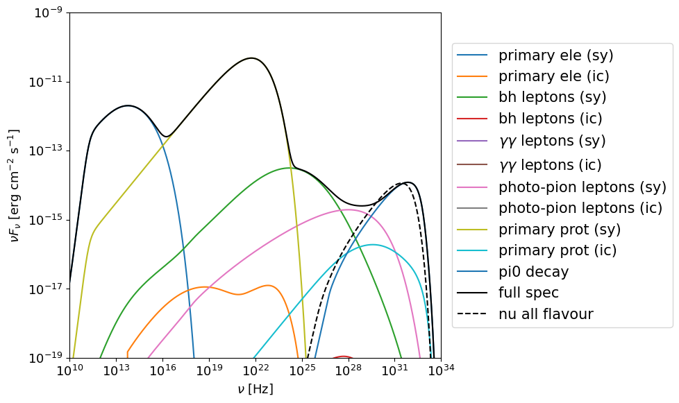
[12]:
plt.figure(figsize = [10, 6])


matplotlib.rcParams.update({'font.size': 13})

names = ['full spec', 'primary ele (sy)', 'primary ele (ic)', 'bh leptons (sy)', 'bh leptons (ic)', r'$\gamma \gamma$ leptons (sy)',
         r'$\gamma \gamma$ leptons (ic)', 'photo-pion leptons (sy)', 'photo-pion leptons (ic)', 'primary prot (sy)', 'primary prot (ic)','pi0 decay']

for i in range(len(Lobs)-1):
    plt.plot(grid_gammas_plot, Lobs[i+1], alpha = 1.0, label = names[i+1])

i = 0
plt.plot(grid_gammas_plot, Lobs[i], alpha = 1.0, label = names[i], color = 'k', ls = '-')
plt.plot(grid_neutrinos_plot, Nu_Lobs, alpha = 1.0, label = 'nu all flavour', color = 'k', ls = '--')

plt.ylim([1e-19 ,1e-9])
plt.xlim([1e10, 1e34])
plt.ylabel(r'$\nu F_{\nu}$ [erg $\mathrm{cm^{-2} \ s^{-1}}$]')
plt.xlabel(r'$\nu$ [Hz]')
plt.xscale('log')
plt.legend(fontsize = 15, bbox_to_anchor = [1.01, 0.5], loc = 'center left')
plt.yscale('log')
#plt.legend(loc = 'upper left', fontsize = 16)
#plt.savefig('proton_synchrotron_decomposed_am3.png', dpi=300, bbox_inches = 'tight')
plt.tight_layout()
plt.show()
[ ]: