Adding your own terms
This notebook shows how to add custom terms to the transport equation that AM³ solves (eq. 6 in Klinger et al. 2024):
where
and the extra cooling term: \(t_{extra\;cooling}^{-1}(E)=\dfrac{\dot{E}(E)}{E}\) can be inserted via am3.set_t_<species>_extra_cooling(array)
and the escape term: \(t_{escape}^{-1}(E) = \alpha(E)\) can be inserted via am3.set_t_<species>_escape(array)
and the injection term: \(Q(E)\) can be inserted via am3.set_injection_rate_<species>(array)
[1]:
import numpy as np
import matplotlib.pyplot as plt

# %matplotlib widget

from tqdm import trange
import am3 as am3lib
[2]:
# Some useful definitions
c_light=3.e10              # speed of light--always useful
m_electron=9.10938356e-28  # electron mass
sigma_t=6.65e-25           # Thomson cross section
mec2 = m_electron*c_light**2
eV2erg = 1.60218e-12
erg2eV = 1/eV2erg
set up two AM³ instances, one for testing the escape term and one for the extra cooling term
[3]:
def get_AM3(escape=0):
    am3 = am3lib.AM3()
    am3.update_energy_grid(1e-6, 1e3, 1e22)
    # set switches
    am3.set_estimate_max_energies(0)

    am3.set_process_parse_sed(1)
    am3.set_process_hadronic(1)
    am3.set_process_merge_positrons_into_electrons(0)
    am3.set_process_escape(escape)
    # expansion related
    am3.set_process_adiabatic_cooling(0)
    am3.set_process_expansion(0)

    # synchrotron related
    am3.set_process_electron_syn(0)
    am3.set_process_electron_syn_emission(0)
    am3.set_process_electron_syn_cooling(0)
    am3.set_process_quantum_syn(0)
    am3.set_process_ssa(0)
    am3.set_process_proton_syn(0)
    am3.set_process_proton_syn_emission(0)
    am3.set_process_proton_syn_cooling(0)
    am3.set_process_pion_syn(0)
    am3.set_process_pion_syn_emission(0)
    am3.set_process_pion_syn_cooling(0)
    am3.set_process_muon_syn(0)
    am3.set_process_muon_syn_emission(0)
    am3.set_process_muon_syn_cooling(0)

    # inverse Compton related
    am3.set_process_electron_compton(0)
    am3.set_process_electron_compton_emission(0)
    am3.set_process_electron_compton_cooling(0)
    am3.set_process_compton_photon_energy_loss(0)
    am3.set_process_proton_compton(0)
    am3.set_process_proton_compton_emission(0)
    am3.set_process_proton_compton_cooling(0)
    am3.set_process_pion_compton(0)
    am3.set_process_pion_compton_emission(0)
    am3.set_process_pion_compton_cooling(0)
    am3.set_process_muon_compton(0)
    am3.set_process_muon_compton_emission(0)
    am3.set_process_muon_compton_cooling(0)

    # secondary decay
    am3.set_process_pion_decay(0)
    am3.set_process_muon_decay(0)

    # pair production (gamma+gamma -> e- + e+)
    am3.set_process_annihilation(0)
    am3.set_process_annihilation_cooling(0)
    am3.set_process_annihilation_pair_emission(0)

    # Bethe-Heitler
    am3.set_process_bethe_heitler(0)
    am3.set_process_bethe_heitler_emission(0)
    am3.set_process_bethe_heitler_cooling(0)

    # p-gamma
    am3.set_process_photopion(0)
    am3.set_process_photopion_emission(0)
    am3.set_process_photopion_cooling(0)
    am3.set_process_photopion_photon_loss(0)

    # proton proton
    am3.set_process_pp(0)
    am3.set_process_pp_emission(0)
    am3.set_process_pp_emission_pi0_into_cascade(0)
    am3.set_process_pp_cooling(0)
    return am3

am3_esc = get_AM3(escape=1)
am3_cool = get_AM3(escape=0)
[4]:
am3_esc.init_kernels()
am3_cool.init_kernels()
init. AM3 kernels:
AM3 has the following switches (at step: 0)
estimate maximum energies: 0
parse sed components: 1
escape: 1
expansion: 0
adiabatic: 0
synchrotron:
  e+/-: 0  (em..: 0, cool.: 0)
  protons:0  (em..: 0, cool.: 0)
  pions:0  (em..: 0, cool.: 0)
  muons:0  (em..: 0, cool.: 0)
  syn-self-abs.:0
  e+/- quantum-syn.:0
inv. Compton:
  e+/-: 0  (em.. : 0, cool.: 0 (continuous))
  photon loss due to upscattering: 0
  protons:0  (em.. (step approx.): 0, no cooling)
  pions:0  (em.. (step approx.): 0, cont. cool.: 0)
  muons:0  (em.. (step approx.): 0, cont. cool.: 0)
pair prod. (gamma+gamma->e+e)0  (photon loss.: 0, e+/- source (feedback): 0(opt. 14-bin kernel))
'hadronic' processes (below): 1
 Pion decay: 0 Muon decay:0)
proton Bethe-Heitler: 0  (em..: 0, cool.: 0)
proton photo-pion: 0  (em..: 0, cool.: 0, photon loss: 0)
proton p-p: 0  (em..: 0 , cool.: 0)

AM3 params (comoving):
escape_timescale: 1e+06 s
  with fractions: (protons: 1, neutrons: 1, pions: 1, muons: 1, neutrinos: 1, pairs: 1)
expansion_timescale: 1e+06 s
t_adi: 3e+06 s
B: 0.01 G
pp target density = 0 cm^-3
dt = 1000 s
eta_Bohm: electrons:1, protons: 1
inj. el:
  power density = 0 erg/s/cm^3,
   Emin = 1e+07 eV,
   Ebreak = 1e+07 eV,
   Emax = 1e+13 eV,
   index = 2,
   index above break = 2,
   cut_off steepness = 1
inj. protons: power density = 0 erg/s/cm^3,
   Emin = 1e+10 eV,
   Ebreak = 1e+10 eV,
   Emax = 1e+15 eV,
   index = 2,
   index above break = 2,
   cut_off steepness = 1

init. AM3 kernels:
AM3 has the following switches (at step: 0)
estimate maximum energies: 0
parse sed components: 1
escape: 0
expansion: 0
adiabatic: 0
synchrotron:
  e+/-: 0  (em..: 0, cool.: 0)
  protons:0  (em..: 0, cool.: 0)
  pions:0  (em..: 0, cool.: 0)
  muons:0  (em..: 0, cool.: 0)
  syn-self-abs.:0
  e+/- quantum-syn.:0
inv. Compton:
  e+/-: 0  (em.. : 0, cool.: 0 (continuous))
  photon loss due to upscattering: 0
  protons:0  (em.. (step approx.): 0, no cooling)
  pions:0  (em.. (step approx.): 0, cont. cool.: 0)
  muons:0  (em.. (step approx.): 0, cont. cool.: 0)
pair prod. (gamma+gamma->e+e)0  (photon loss.: 0, e+/- source (feedback): 0(opt. 14-bin kernel))
'hadronic' processes (below): 1
 Pion decay: 0 Muon decay:0)
proton Bethe-Heitler: 0  (em..: 0, cool.: 0)
proton photo-pion: 0  (em..: 0, cool.: 0, photon loss: 0)
proton p-p: 0  (em..: 0 , cool.: 0)

AM3 params (comoving):
escape_timescale: 1e+06 s
  with fractions: (protons: 1, neutrons: 1, pions: 1, muons: 1, neutrinos: 1, pairs: 1)
expansion_timescale: 1e+06 s
t_adi: 3e+06 s
B: 0.01 G
pp target density = 0 cm^-3
dt = 1000 s
eta_Bohm: electrons:1, protons: 1
inj. el:
  power density = 0 erg/s/cm^3,
   Emin = 1e+07 eV,
   Ebreak = 1e+07 eV,
   Emax = 1e+13 eV,
   index = 2,
   index above break = 2,
   cut_off steepness = 1
inj. protons: power density = 0 erg/s/cm^3,
   Emin = 1e+10 eV,
   Ebreak = 1e+10 eV,
   Emax = 1e+15 eV,
   index = 2,
   index above break = 2,
   cut_off steepness = 1
[5]:
# short cuts for energy grids
Ep_eV = am3_esc.get_egrid_had()
Ep_erg = Ep_eV * eV2erg
[6]:
def powerlaw_array_number(Es, Emin, Emax, p, norm):
    powerlaw = (Es/Emin)**(-p) * np.less_equal(Es, Emax) * np.greater_equal(Es, Emin) #np.exp(-(Es/Emax))
    integral = np.log(Es[1]/Es[0]) * np.sum(Es * powerlaw)
    return norm/integral * powerlaw
set a continuous injection term with a constant rate as a power law with a broad energy range
[7]:
Emin = 1e10
Emax = 1e20
s_inj = 2
N0 = 1

am3_esc.clear_particle_densities()
am3_esc.set_injection_rate_protons(Ep_eV * powerlaw_array_number(Ep_eV, Emin, Emax, s_inj, N0))

am3_cool.clear_particle_densities()
am3_cool.set_injection_rate_protons(Ep_eV * powerlaw_array_number(Ep_eV, Emin, Emax, s_inj, N0))
[8]:
fig, ax = plt.subplots()

ax.loglog(Ep_eV,  Ep_erg*am3_cool.get_injection_rate_protons())
ax.set_aspect("equal")
ax.grid(alpha=0.3)
ax.set_ylim(1e-5, 1e5)
ax.set_xlabel(r"$E$ [eV]")
ax.set_ylabel(r"$E dN/dEdVdt$ [erg/cm³s]")
ax.set_title("proton injection term")
ax.set_aspect("equal")

define an (unphysical) time scale array for the escape/extra coooling term to test the implementation
[9]:
t_escape = 10**(np.sin(np.log10(Ep_erg)) + 2) # in seconds
t_advect = 10**(np.sin(np.log10(Ep_erg)+3) + 2)  # in seconds
t_step = 10 # in seconds
Ntotal = int(1e4/t_step)

am3_esc.set_t_proton_escape(t_escape)
am3_cool.set_t_proton_extra_cooling(t_advect)
am3_esc.set_solver_time_step(t_step)
am3_cool.set_solver_time_step(t_step)
[10]:
fig, ax = plt.subplots()
ax.axvspan(Emin, Emax, alpha=0.3, label="injection energy range")
ax.loglog(Ep_eV, am3_esc.get_t_proton_escape(), label="escape array")
ax.loglog(Ep_eV, am3_cool.get_t_proton_extra_cooling(), label="extra cooling")
ax.axhline(t_step, ls="--", label="time step", c="tab:red")
ax.axhline(Ntotal*t_step, ls="--", label="total simulation time", c="k")
ax.legend()
ax.set_aspect("equal")
ax.grid(alpha=0.3)
ax.set_ylim(1e-3, 1e5)
ax.set_xlabel(r"$E$ [eV]")
ax.set_ylabel(r"$t$ [s]")
ax.set_title("proton timescales")
ax.set_aspect("equal")

run both simulations
[11]:
am3_esc.clear_particle_densities()
am3_esc.clear_particle_densities()
for i in trange(Ntotal):
    am3_esc.evolve_step()
    am3_cool.evolve_step()
100%|██████████| 1000/1000 [00:00<00:00, 2621.65it/s]
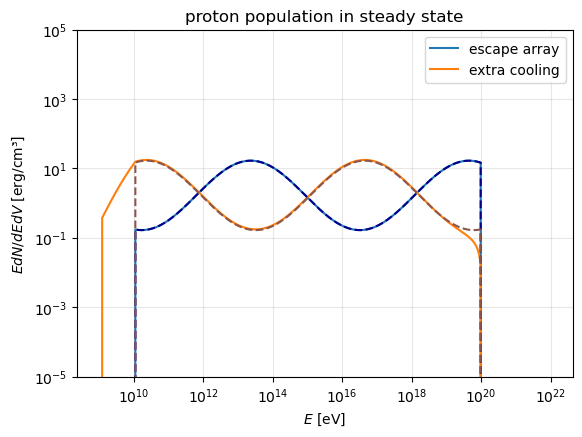
plot the final proton distribution and compare it to the steady-state expectation \(n_{steady\; state} \to Q(E) t_{escape/extra\;cooling}\)
[12]:
fig, ax = plt.subplots()

ax.loglog(Ep_eV, Ep_erg*am3_esc.get_protons(), label="escape array")
ax.loglog(Ep_eV, Ep_erg*am3_cool.get_protons(), label="extra cooling")
ax.loglog(Ep_eV, Ep_erg*am3_esc.get_injection_rate_protons()*am3_esc.get_t_proton_escape(), ls="--", c="darkblue")
ax.loglog(Ep_eV, Ep_erg*am3_cool.get_injection_rate_protons()*am3_cool.get_t_proton_extra_cooling(), ls="--", c="tab:brown")
ax.legend()
ax.set_aspect("equal")
ax.grid(alpha=0.3)
ax.set_ylim(1e-5, 1e5)
ax.set_xlabel(r"$E$ [eV]")
ax.set_ylabel(r"$E dN/dEdV$ [erg/cm³]")
ax.set_title("proton population in steady state")
ax.set_aspect("equal")