Example 3: Tidal disruption event (TDE) simulation
Simplified example in Python for modeling isotropic electromagnetic cascade and neutrino emission from tidal disruption events (TDEs).
Model based on Yuan, Winter and Lunardini, ApJ 969 (2024).
If using this TDE model, please cite the above paper additionally to AM3.
1. Import packages and define the physical constants
[1]:
import numpy as np
import matplotlib.pyplot as plt
import sys
sys.path.append('/path to AM3 library/')
import am3

c0 = 3e10 # speed of light
Msun = 2e33 #solar mass in grams
pc2cm = 3.08e18 # pc to cm
k_Boltzmann = 8.6e-5 # eV/K, convert K to eV
eV2Hz = 2.4e14 # convert eV to Hz
Jy2CGS = 1e-23 # 1 Jy = 1e-23 erg/s/cm^2/Hz
protonmass = 1.67e-24 # proton mass in g
elecmass = 9.1e-28 # electron mass in g
d2s = 24*3600.0 # day to s
erg2GeV = 624.15 # erg to GeV
ElecStatic = 4.8e-10 # electron charge
2. Define a class for generating external photon spectra
[2]:
class ExtPH:
    '''
    set_external_G_spec(Obs_time, radius, Elist, corrected_lu, timelist, Ebb)
    input: time in observer's frame, radius of the radiaton zone, energy array for external photon spectra,
           bolometric luminosity array, time array for luminosity, black body energy
    output: external photon rate spectra dN/dlogE/dt[cm^-3 s^-1]
    '''
    @classmethod
    def BlackBodySpec(cls, Energy, Temp0): #in eV, return in arbitrary units, dn/dlnE
        theta = Energy / Temp0
        tt = np.array(np.exp(theta), dtype = float)
        np.clip(tt, 1e-50, 1e100)
        spec = 1 / (tt - 1)
        if hasattr(Energy, "__len__"):
            spec[spec < 1e-20] = 0
        return spec * Energy**3


    @classmethod
    def set_external_G_spec(cls, Obs_time, radius, Elist, corrected_lu, timelist, Ebb):
        IntegralFlux = linear_interpolation(Obs_time, timelist, corrected_lu)
        EnergyUp = Ebb * 1e6
        EnergyLow = Ebb / 1e6
        dLogE = np.log(EnergyUp / EnergyLow) / 200
        EnergyList = np.exp(np.arange(np.log(EnergyLow), np.log(EnergyUp), dLogE))
        dEnergy = EnergyList * np.exp(dLogE) - EnergyList
        integral = sum(dEnergy * cls.BlackBodySpec(EnergyList, Ebb))
        return  IntegralFlux / integral * cls.BlackBodySpec(Elist/(1+redshift), Ebb) / (4*np.pi/3*radius**3) * erg2GeV * 1e9/3

def linear_interpolation(x, index_array, interp_array):
    '''
    1D linear interpolation
    input: x, x-array, y-array
    '''
    length = len(index_array)
    if len(index_array) != len(interp_array):
        print ("Interpolation error!")
        return 0

    elif (x < index_array[0]) or x > (index_array[length-1]):
        return 0
    else:
        for i in range(length-1):
            if x <= index_array[i+1] and x >= index_array[i]:
                return interp_array[i] + (interp_array[i+1] - interp_array[i])/(index_array[i+1] - index_array[i]) * (x - index_array[i])
3. Initialize AM3 and set the switches
See https://am3.readthedocs.io/en/latest/examples/blazar_detailed_example.html for a more complete usage of the switches.
[ ]:
am3 = am3.AM3()

Eg_eV = am3.get_egrid_photons() #energy grid for photons
En_eV = am3.get_egrid_neutrinos() #energy grid for neutrinos

am3.set_estimate_max_energies(1)
am3.set_process_parse_sed(1)
am3.set_process_hadronic(1)
am3.set_process_merge_positrons_into_electrons(0)
am3.set_process_escape(1)
am3.set_process_expansion(0)
am3.set_process_adiabatic_cooling(0)
am3.set_process_electron_syn(1)
am3.set_process_ssa(1)
am3.set_process_proton_syn(1)
am3.set_process_quantum_syn(0)
am3.set_process_electron_compton(1)
am3.set_process_proton_compton(1)
am3.set_process_compton_photon_energy_loss(0)

am3.set_process_muon_syn(1)
am3.set_process_pion_syn(1)
am3.set_process_muon_compton(1)
am3.set_process_pion_compton(1)
am3.set_process_pion_decay(1)
am3.set_process_muon_decay(1)

am3.set_process_annihilation(1)
am3.set_optimize_annihilation_pair_emission(1)

am3.set_process_bethe_heitler(1)
am3.set_optimize_bethe_heitler_outgoing_pairs_grid(1)
am3.set_optimize_bethe_heitler_incoming_protons_min(1e12)
am3.set_optimize_bethe_heitler_target_photon_max(1e6)

am3.set_process_photopion(1)
am3.set_optimize_photopion_target_photon_grid(1)
am3.set_optimize_photopion_target_photon_max(1e6)

am3.init_kernels()
4. Define simulation parameters
[4]:
t_start = -250 # start time t-t_pk in observer's frame
t_obs_nu = 370 # neutrino detection time in observer's frame
t_stop = t_obs_nu + 20 # time to stop the simulation
redshift = 0.995 # redshift
LuminDistance = 8.45e9 * pc2cm # luminosity distance in cm

E_OUV = 1.38 # peak energy of OUV black body spectra [eV]
L_OUV = np.array([2.85e44, 3.47e45, 6.51e45, 1.80e46, 1.37e46, 8.43e45, 2.08e45]) #bolometric OUV luminosities
T_OUV = np.array([-280, -183, -148, 0.0, 172, 350, 1197]) #time list for the bolometric OUV luminosities

E_X = 72 # peak energy of X-ray black body spectra [eV]
L_X = np.array([3.40e45, 3.40e45]) #bolometric X-ray luminosities
T_X = np.array([-200, 600]) #time list for the bolometric X-ray luminosities

E_IR = 0.16 # peak energy of IR black body spectra [eV]
L_IR = np.array([1.85e44, 1.76e45, 2.93e45, 3.87e45, 3.88e45, 3.87e45, 3.71e45, 3.45e45, 3.12e45, 2.38e45]) #bolometric IR luminosities
T_IR = np.array([-250, -122, -56, 0, 58, 142, 250, 470, 630, 810]) #time list for the bolometric IR luminosities

SMBHmass = 1e8 * Msun # SMBH mass in g
Starmass = 1.0 * Msun # mass of disrupted star in g
L_Edd = 1.3e45 * SMBHmass / (1e7 * Msun) # Eddington Luminosity
SuperEddingtonParam = 100 *7.0/18 # M_acc / L_Edd at t_peak
eta_p = 0.2 # proton efficiency
SpecIndex = 2.0 # proton spectral index

L_p = SuperEddingtonParam * eta_p * L_Edd * L_OUV/max(L_OUV) # proton luminosity

runtime = t_start # record current run time

radius = 5e17 # radius of the dust torus
fracdt = 0.01 # time step = fracdt * R / c
Epmax = 1.5e9 * 1e9 # proton maximum energy in SMBH rest frame
5. Run the simulation from t_start to t_stop in a loop
[5]:
while runtime < t_stop:
    '''
    set the runtimes and time steps
    '''
    T_rest = runtime / (1+redshift) # SMBH rest frame time
    mag_B = 0.1 # set magnetic field to 0.1 Gauss

    time0 = runtime
    t_esc = radius / c0
    am3.set_escape_timescale(radius / c0) #free streaming time
    delta_runtime = min(fracdt * t_esc/d2s,  1) * (1 + redshift) # control the time step to not exceed 1 day


    am3.set_solver_time_step(min(fracdt * t_esc, 24*3600)) # solver time step in seconds
    runtime += delta_runtime


    '''
    set external photon spectra
    '''
    spec_extG = ExtPH.set_external_G_spec(runtime, radius, Eg_eV, L_OUV, T_OUV, E_OUV) +  ExtPH.set_external_G_spec(runtime, radius, Eg_eV, L_X, T_X, E_X) + ExtPH.set_external_G_spec(runtime, radius, Eg_eV, L_IR, T_IR, E_IR)

    am3.set_injection_rate_photons(spec_extG)

    '''
    set magnetic field and inject protons
    '''
    am3.set_mag_field(mag_B)

    volume = (4*3.14/3*radius**3)
    pro_luminosity = linear_interpolation(runtime, T_OUV, L_p)
    p_inj_Emin_eV = 1e9
    p_inj_Emax_eV = Epmax
    p_inj_index = SpecIndex

    am3.set_powerlaw_injection_parameters_protons(volume, pro_luminosity, p_inj_Emin_eV, p_inj_Emin_eV, p_inj_Emax_eV, p_inj_index, p_inj_index, 1.0)

    '''
    evolve the system by one time step
    '''
    am3.evolve_step()


    '''
    convert the spectra for photon components and neutrinos to the observer's frame and obtain the SEDs at neutrino detection time t_obs_nu
    '''

    if t_obs_nu < runtime and t_obs_nu >= time0:

        '''
        cascade photon spectra
        '''
        spec_const = Eg_eV/1e9/erg2GeV  * c0 * radius**2/(LuminDistance**2)  #
        energy = Eg_eV  / (1 + redshift) # eV
        dataG = np.transpose([energy, spec_const * am3.get_photons(),
                            spec_const * (am3.get_photons_injected_electrons_syn()),
                            spec_const * (am3.get_photons_injected_electrons_compton()),
                            spec_const * am3.get_photons_bethe_heitler_pairs_syn_compton(),
                            spec_const * am3.get_photons_annihilation_pairs_syn_compton(),
                            spec_const * am3.get_photons_photo_pion_pairs_syn_compton(),
                            spec_const * am3.get_photons_protons_syn_compton(),
                            spec_const * am3.get_photons_pi0_decay()
                            ])


        '''
        external photon spectrum
        '''
        dataext = np.transpose([energy, spec_const*spec_extG*4*3.14/3 * radius/c0])


        '''
        neutrino spectrum
        '''
        spec_const = En_eV/1e9/erg2GeV * c0 * radius**2/(LuminDistance**2)  #
        energy = En_eV / (1 + redshift) # eV
        dataNu = np.transpose([energy, spec_const * am3.get_neutrinos_photopion()])
/var/folders/25/d230kxr90hj414fnx8hg1f_4000956/T/ipykernel_82300/1259833014.py:11: RuntimeWarning: overflow encountered in exp
  tt = np.array(np.exp(theta), dtype = float)
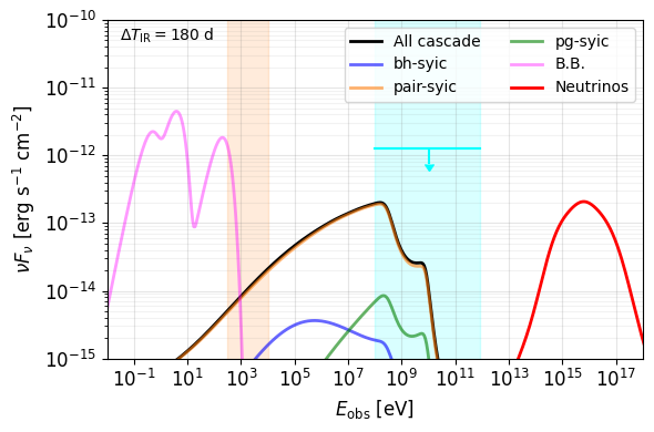
6. Plot the multi-wavelength and neutrino SEDs
Cf. Fig 3 of Yuan, Winter and Lunardini 2024 (https://arxiv.org/pdf/2401.09320).
[6]:
plt.figure(figsize=(6,4))

plt.fill_between([300,1e4], [1e-20,1e-20], [1,1], color = "C1", alpha = 0.15)
plt.fill_between([1e8,8e11], [1e-20,1e-20], [1,1], color = "cyan", alpha = 0.15)

data=dataG
datacas = data[:,4] + data[:,5] + data[:,6] + data[:,7] + data[:,8]
plt.plot(data[:,0], datacas, lw=2, color = "k", label = "All cascade")
plt.loglog(data[:,0], data[:,4], lw=2,color = "blue", alpha=0.6, label = r"bh-syic")
plt.loglog(data[:,0], data[:,5], lw=2,color = "C1",alpha=0.6, label = r"pair-syic")
plt.loglog(data[:,0], data[:,6], lw=2,color = "green",alpha=0.6, label = r"pg-syic")
plt.ylim(1e-15,1e-10)
plt.xlim(1e-2,1e18)

data = dataext
plt.loglog(data[:,0], data[:,1], lw=2, color = "magenta", alpha=0.4,label = r"B.B.")

data=dataNu
plt.loglog(data[:,0], data[:,1], color = "red", lw=2, label = r"Neutrinos")

plt.legend(ncol=2)

plt.grid(color="gray", alpha = 0.1, which="minor")
plt.grid(color="gray", alpha = 0.2, which="major")

plt.xlabel(r"$E_{\rm obs}$ [eV]", fontsize=12)
plt.ylabel(r"$\nu F_\nu~[\rm erg~s^{-1}~cm^{-2}]$", fontsize=12)

plt.xticks(10.0**(1+2*np.arange(-1,9)), fontsize=12)
plt.yticks(fontsize=12)

plt.plot([1e8, 8e11], [1.25e-12, 1.25e-12], lw=1.5, color = "cyan")

plt.text(3e-2, 5e-11, r"$\Delta T_{\rm IR}=180$ d")

plt.errorbar([1e10],[1.25e-12], xerr=[[1e10-1e8], [8e11-1e10]], yerr=[[5e-13], [7e-12]], uplims=True, color = "cyan")
plt.arrow(1.06e14, 3e-13, 0, -2e13, color="red")
plt.tight_layout()

plt.show()
[ ]: